What is Unsupervised Learning?
Unsupervised learning is where you only have input data (X) and no corresponding output variables.The goal for unsupervised learning is to model the underlying structure or distribution in the data in order to learn more about the data. Thus as we don’t have the class-labels(the output classes for the input data), algorithms are left to their own formulations to discover and present the interesting structure in the data. Thus the algorithms try to find some similarity or some kind of association between the input data, and try to seperate or cluster the data that are similar to each other.
Applications of Unsupervised Learning:
Social Media Analysis–> People belonging to the same regions of interest can be recommended with products of their interest. Similarly indirectly associated people can be recommended to each other.
Association–> We can recommend products that are generally bought together. For eg: we can keep bread and butter together as people tend to buy them together.
In this blog we will learn about the K-means clustering algorithm which is one of the most widely used unsupervised machine learning algorithms.
People are often confused between KNN(K- nearest neighbours) which is a supervised learning algorithm and K-means algorithm. Lets understand both of them in a very simple way.
KNN(K-Nearest Neighbours) Algorithm
KNN algorithm is one of the simplest classification algorithm and it is one of the most used learning algorithms. Since its a supervised algorithm, it classifies the data into the class labels according to the input data. For eg, the iris dataset will be plotted according to the class labels something like :

Now lets say that we have a new input point, and we want to know which class does it belong to. Now this point will be plotted on the graph accoring to its input values. Now we will check to which class is the point nearest to.But how do we check the proximity?? We simply calculate the Euclidean Distance between the new point and an existing point. If the distance between the new and existing point is minimum, then the new point will belong to the class of the existing point.
But how many such points should be consider for calculating the distance. This depends the chosen value of K.
How do we choose K?
There is no fixed value of K that gives an optimal solution. We should always iterate over some values of K(preferably (1-21)), and check the accuracy of the model. The value of K of the model with the highest or the most stable accuracy must be chosen.
For K=1: Lets say we choose K=1, and we have 3 labeled classes. This is the simplest scenario. Let x be the point to be labeled. Find the point closest to x . Let it be y. Now nearest neighbor rule asks to assign the label of y to x.
For K=5: This is a straightforward extension of 1NN. Basically what we do is that we try to find the k nearest neighbor and do a majority voting.k = 5 and there are 4 instances of C1 and 1 instance of C2. In this case , KNN says that new point has to labeled as C1 as it forms the majority. We follow a similar argument when there are multiple classes.

This is all about the KNN Algorithm.
Pros:
- Very easy to understand and implement. A k-NN implementation does not require much code and can be a quick and simple way to begin machine learning datasets.
- Does not assume any probability distributions on the input data. This can come in handy for inputs where the probability distribution is unknown and is therefore robust.
Cons:
- Sensitive to localized data. Since k-NN gets all of its information from the input’s neighbors, localized anomalies affect outcomes significantly, rather than for an algorithm that uses a generalized view of the data.
K-Means Algorithm
K-means clustering is a type of unsupervised learning.The goal of this algorithm is to find groups in the data, with the number of groups represented by the variable K. The algorithm works iteratively to assign each data point to one of K groups based on the features that are provided. Data points are clustered based on feature similarity.
Difference b/w KNN and K-Means: The K in KNN is the number of neighbouring points, while that in K-Means is the number of custers.
Algo:
-
The algorithm inputs are the number of clusters Κ and the data set. The data set is a collection of features for each data point.
-
The algorithms starts with initial estimates for the Κ centroids, which can either be randomly generated or randomly selected from the data set.
-
The algorithm inputs are the number of clusters Κ and the data set. The data set is a collection of features for each data point.
-
The algorithms starts with initial estimates for the Κ centroids, which can either be randomly generated or randomly selected from the data set.
-
Each centroid defines one of the clusters. In this step, each data point is assigned to its nearest centroid, based on the squared Euclidean distance.
- The centroids are recomputed. This is done by taking the mean of all data points assigned to that centroid’s cluster.
- The algorithm iterates between the last 2 steps until a stopping criteria is met (i.e., no data points change clusters, the sum of the distances is minimized, or some maximum number of iterations is reached).
Choosing K
The algorithm described above finds the clusters and data set labels for a particular pre-chosen K. To find the number of clusters in the data, the user needs to run the K-means clustering algorithm for a range of K values and compare the results. In general, there is no method for determining exact value of K, but an estimate can be made by some metrics.
One of the metrics that is commonly used to compare results across different values of K is the mean distance between data points and their cluster centroid. Since increasing the number of clusters will always reduce the distance to data points, increasing K will always decrease this metric, to the extreme of reaching zero when K is the same as the number of data points. Thus, this metric cannot be used as the sole target. Instead, mean distance to the centroid as a function of K is plotted and the “elbow point,” where the rate of decrease sharply shifts, can be used to roughly determine K.

Lets use K-means using Sklearn.
Importing required packages
from sklearn.cluster import KMeans
import numpy as np
import matplotlib.pyplot as plt
Creating dummy data
X = np.array([[1.1,2.2],[1.6,4.7],[1.3,0],[4.3,2.7],[2.3,4.1],[3.5,0.6],[4.2,3.9],[0.1,0.3],[1.3,1.5],[2.1,2.5],[5.9,1.9],[1.4,3.3],[3.1,1.3],[2,4],[1,5],[3,6],[5.7,3],[2,1],[2,5.2],[3,4],[3,2.7],[2.3,4.2],[1.1,1.3],[1.3,2.1],[2.1,2.3],[3.1,2.7],[3.1,1.3],[4.5,3.4],[4.1,4],[4.7,3],[4.2,3.6],[3.9,4.2]])
a=[]
b=[]
for i in list(X):
    a.append(i[0])
    b.append(i[1])
Plotting the input data
plt.scatter(a,b)
plt.title('Unclustered Data')
plt.show()
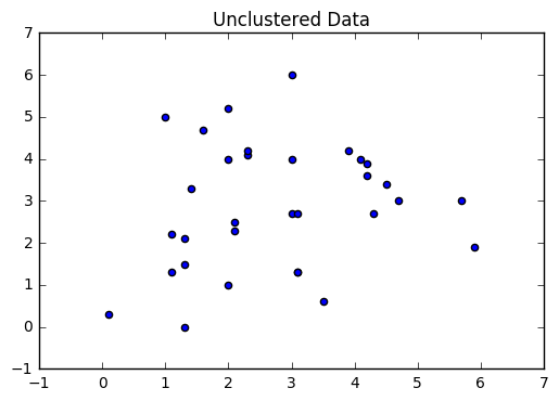
We can see that originally all the input points are unclassified, i.e they belong to the same class. Now we will divide them into clusters.
Using the inbuilt K-means function.
kmeans = KMeans(n_clusters=2, random_state=0) #number of clusters=2
kmeans.fit(X)# fitting the data into the algorithm
KMeans(algorithm='auto', copy_x=True, init='k-means++', max_iter=300,
    n_clusters=2, n_init=10, n_jobs=1, precompute_distances='auto',
    random_state=0, tol=0.0001, verbose=0)
kmeans.labels_ #showing the predicted labels for the input data
array([0, 1, 0, 1, 1, 0, 1, 0, 0, 0, 1, 0, 0, 1, 1, 1, 1, 0, 1, 1, 1, 1, 0,
       0, 0, 1, 0, 1, 1, 1, 1, 1], dtype=int32)
As we had chosen K=2, the algorithm has classified the data points into cluster’s 0 and 1.
kmeans.predict([[0, 0], [4, 4]]) #predicting the labels for new input data
array([0, 1], dtype=int32)
kmeans.cluster_centers_ # the centers of the newly formed clusters
array([[ 1.80769231,  1.51538462],
       [ 3.41052632,  3.80526316]])
Cluster = kmeans.labels_
centers = kmeans.cluster_centers_
fig = plt.figure()
ax = fig.add_subplot(111)
scatter = ax.scatter(a,b,c=Cluster,s=30)
for i,j in centers:
    ax.scatter(i,j,s=50,c='red',marker='x')
ax.set_xlabel('x')
ax.set_ylabel('y')
plt.colorbar(scatter)
plt.title('Clusters = %s'%(kmeans.cluster_centers_.shape[0]))
plt.show()
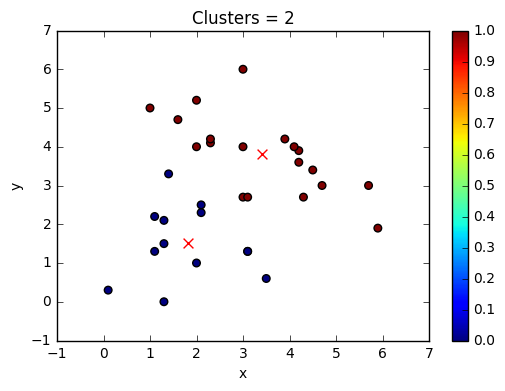
The above plot shows data clustered into 2 classes. Lets try K=4.
kmeans = KMeans(n_clusters=4, random_state=0)
kmeans.fit(X)
print('Labels for K=4:  ',kmeans.labels_)
print('Cluster Centres for K=4:  ',kmeans.cluster_centers_ )
Cluster = kmeans.labels_
centers = kmeans.cluster_centers_
fig = plt.figure()
ax = fig.add_subplot(111)
scatter = ax.scatter(a,b,c=Cluster,s=30)
for i,j in centers:
    ax.scatter(i,j,s=50,c='red',marker='x')
ax.set_xlabel('x')
ax.set_ylabel('y')
plt.colorbar(scatter)
plt.title('Clusters = %s'%(kmeans.cluster_centers_.shape[0]))
plt.show()
Labels for K=4:   [2 0 2 3 0 1 3 2 2 1 3 0 1 0 0 0 3 2 0 0 1 0 2 2 1 1 1 3 3 3 3 3]
Cluster Centres for K=4:   [[ 2.06666667  4.5       ]
 [ 2.85714286  1.91428571]
 [ 1.17142857  1.2       ]
 [ 4.61111111  3.3       ]]
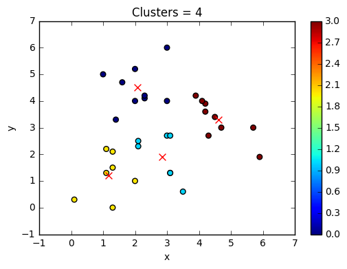
We can clearly see that the points are now shifted to other clusters depending upon the distance from the centroids.
from scipy.spatial.distance import cdist
distortions = []
K = range(1,10)
for k in K:
    kmeanModel = KMeans(n_clusters=k).fit(X)
    kmeanModel.fit(X)
    distortions.append(sum(np.min(cdist(X, kmeanModel.cluster_centers_, 'euclidean'), axis=1)) / X.shape[0])
plt.plot(K, distortions,marker='o')
plt.xlabel('k')
plt.ylabel('Average within-cluster distance to centroid')
plt.title('The Elbow Method')
plt.show()
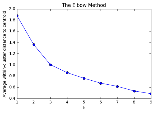
We can see that the variance reduces significantly from 2 to 3. Thus the number of clusters can be 3 or 4.
There are many other Unsupervised learning algorothims other than clustering. Following are some resources that will be helpful in learning them:
1) Different Unsupervised Learning algorithms
2) Apriori Algorithm (Association)
4) Dimensionality Reduction and PCA
5) Topic Modeling and LDA (Text Analysis and NLP)
6) DBSCAN