Background
Up until now we have seen the typical working of a machine learning algorithm. We learn a function f to map input X (independent features) to output Y (dependent label) with minimum loss on the test data.
Y = f(X) + error
Training: machine learns f from labeled training data
Testing: machine predicts Y from unlabeled testing data
The data we get from real world is messy and thus it becomes difficult to learn f. We need a model that is robust as well as flexible. A model that can be used to solve language as well as vision problems and can also be used in game playing to simulate real-world scenarious.
The learning techniques we have covered do well when the data we are working with is not insanely complex, but it’s not clear how they’d generalize to scenarios like these.
Deep learning, a part of Machine Learning, is really good at learning f, particularly in situations where the data is complex. In fact, Artificial Neural Networks (ANN) are known as universal function approximators because they’re able to learn any function, no matter how vague the dataset is.
What is a neural network ?
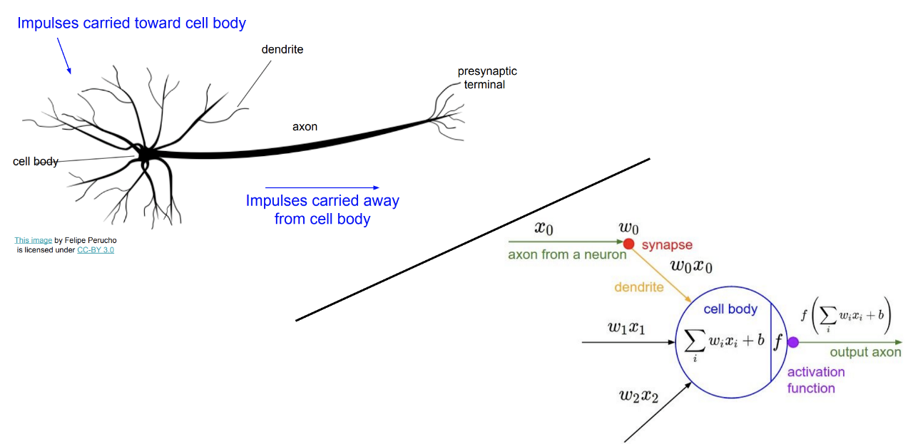
To understand neural networks, let’s first explore the inspiration behind ANN - our brains. The human brain can be described as a biological neural network — an interconnected web of neurons transmitting elaborate patterns of electrical signals. Dendrites receive input signals and, based on those inputs, fire an output signal via an axon. Or something like that. How the human brain actually works is an elaborate and complex mystery, one that we certainly are not going to attempt to tackle in this blog.
With our elementary understanding of the brain function, we can abstract the aforementioned concept by constructing a set a “Inputs” neurons representing the dendrites, this will take the shape of a grid of pixels. The information is then passed to a “hidden” layer which represents the layers within our brain via axon. Finally, this hidden layer connects to an output layer, the equivalent to the motor neurons which causes us to perform an action.
To understand NN, start with perceptrons at neuralnetworksanddeeplearning.com
Architecture of Neural Network
We will start by understanding some terminologies that make up a neural network.
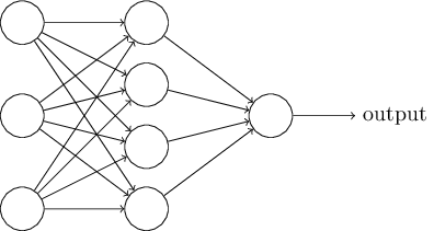
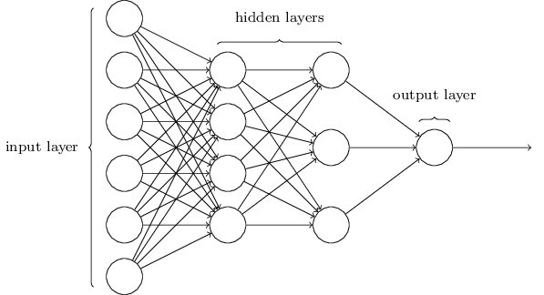
A typical neural network has anything from a few dozen to hundreds, thousands, or even millions of artificial neurons called units arranged in a series of layers, each of which connects to the layers on either side. Some of them, known as input units, are designed to receive various forms of information from the outside world that the network will attempt to learn about, recognize, or otherwise process. Other units sit on the opposite side of the network and signal how it responds to the information it’s learned; those are known as output units. In between the input units and output units are one or more layers of hidden units, which, together, form the majority of the artificial brain. Most neural networks are fully connected, which means each hidden unit and each output unit is connected to every unit in the layers either side. The connections between one unit and another are represented by a number called a weight, which can be either positive (if one unit excites another) or negative (if one unit suppresses or inhibits another). The higher the weight, the more influence one unit has on another. (This corresponds to the way actual brain cells trigger one another across tiny gaps called synapses.)
Such multiple layer networks are sometimes called MultiLayer Perceptrons (MLP), despite being made up of sigmoid neurons, not perceptrons. Learn more about MLPs and how to use them with scikit code at sklearn.neural_network
Working of Neural Network
Again, if we take an analogy with our brain. Brains are made up of neurons which “fire” by emitting electrical signals to other neurons after being sufficiently “activated”. These neurons are malleable in terms of how much a signal from other neurons will add to the activation level of the neuron (vaguely speaking, the weights connecting neurons to each other end up being trained to make the neural connections more useful, just like the parameters in a linear regression can be trained to improve the mapping from input to output).
Taking another example network, a deep neural network looks something like this:
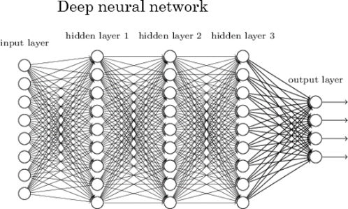
In a gist, this is just a giant mathematical equation with millions of terms and lots of parameters. The input X is, say, a greyscale image represented by a width-by-height matrix of pixel brightnesses. The output Y is a vector of class probabilities. This means we have as an output the probability of each class being the correct label. If this neural net is working well, the highest probability should be for the correct class. And the layers in the middle are just doing a bunch of matrix multiplication by summing activations x weights with non-linear transformations (activation functions) after every hidden layer to enable the network to learn a non-linear function .
Incredibly, you can use gradient descent in the exact same way that we did with linear regression earlier to train these parameters in a way that minimizes loss. So with a lot of examples and a lot of gradient descent, the model can learn how to classify images of animals (for example) correctly. And that, in a nutshell’s nutshell, is “deep learning”.
Information flows through a neural network in two ways. When it’s learning (being trained) or operating normally (after being trained), patterns of information are fed into the network via the input units, which trigger the layers of hidden units, and these in turn arrive at the output units. This common design is called a feedforward network. Not all units “fire” all the time. Each unit receives inputs from the units to its left, and the inputs are multiplied by the weights of the connections they travel along. Every unit adds up all the inputs it receives in this way and (in the simplest type of network) if the sum is more than a certain threshold value, the unit “fires” and triggers the units it’s connected to (those on its right).
Neural networks learn things typically by a feedback process called backpropagation (sometimes abbreviated as “backprop”). This involves comparing the output a network produces with the output it was meant to produce, and using the difference between them to modify the weights of the connections between the units in the network, working from the output units through the hidden units to the input units — going backward, in other words. In time, backpropagation causes the network to learn, reducing the difference between actual and intended output to the point where the two exactly coincide, so the network figures things out exactly as it should.
Once the network has been trained with enough learning examples, it reaches a point where you can present it with an entirely new set of inputs it’s never seen before and see how it responds.
The following MIT videos will provide a comprehensive explanation of the working of NN:

Activation functions
To understand the role of activation functions, let’s recap the working of linear regression and logistic regression.
Linear Regression: The goal of (ordinary least-squares) linear regression is to find the optimal weights that when linearly combined with the inputs result in a model that minimizes the vertical offsets between the target and explanatory variables.
So, we compute a linear combination of weights and inputs.
f(x)= b + x1 * w1 + x2 * w2 + … xn * wn = z
Logistic Regression: We put the input z through a non-linear “activation function” – the logistic sigmoid function where.
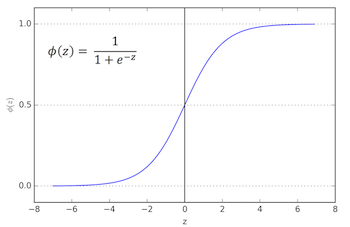
We "squash" the linear net input through a non-linear function, which has the nice property that it returns the conditional probability P(y=1 | x) (i.e., the probability that a sample x belongs to class 1).
Read this Quora answer for better understanding of activation functions.
Further readings:
Cost function
A cost function is a measure of “how good” a neural network did with respect to it’s given training sample and the expected output. It also depends on variables such as weights and biases.
A cost function is a single value, not a vector, because it rates how good the neural network did as a whole.
Specifically, a cost function is of the form
where W is our neural network’s weights, B is our neural network’s biases, Sr is the input of a single training sample, and Er is the desired output of that training sample.
Read this StackOverflow answer to understand the role of cost functions and it’s various types
Backpropagation and gradient checking
We have already mentioned about the information flow in a neural network and introduced the terms “feedforward” and “backprop”. To give a recap:


Read this blog post for a visual explanation of backprop algorithm.
Optimization methods
Once the analytic gradient is computed with backpropagation, the gradients are used to perform a parameter update. There are several approaches for performing the update.
Note that optimization for deep networks is currently a very active area of research. In this section we provide some further pointers for a detailed explanation of various optimization techniques.
Additional Resources
- Andrej Karpathy’s CS231n
- NeuralNetworksandDeepLearning
- All the terms you need to know and an explanation of each term
- Neural Network Glossary
- Play around with the architecture of neural networks with Google’s Neural Network Playground
- Work through at least the first few lectures of Stanford’s CS231n and the first assignment of building a two-layer neural network from scratch to really solidify the concepts covered in this blog.
- Deeplearning.ai - Andrew Ng’s new deep learning course with a comprehensive syllabus on the subject
- Deep Learning Book — foundational, more mathematical
- Fast.ai — less theoretical, much more applied and black box approach
- See Greg Brockman (CTO of OpenAI)’s answer to the question “What are the best ways to pick up Deep Learning skills as an engineer?” on Quora
Example Code
Neural Network code from scratch in Python
As shown during the lecture we will use the XOR problem from Sirajology Python NN Example
import numpy as np
The following is a function definition of the sigmoid function, which is the type of non-linearity chosen for this neural net. It is not the only type of non-linearity that can be chosen, but is has nice analytical features and is easy to teach with. In practice, large-scale deep learning systems use piecewise-linear functions because they are much less expensive to evaluate.
The implementation of this function does double duty. If the deriv=True flag is passed in, the function instead calculates the derivative of the function, which is used in the error backpropogation step.
def nonlin(x, deriv=False):
    if(deriv==True):
        return (x*(1-x))

    return 1/(1+np.exp(-x))
The following code creates the input matrix. Although not mentioned in the video, the third column is for accommodating the bias term and is not part of the input.
#input data

X = np.array([[0,0,1],
            [0,1,1],
            [1,0,1],
            [1,1,1]])
The output of the exclusive OR function follows.
#output data
y = np.array([[0],
             [1],
             [1],
             [0]])
The seed for the random generator is set so that it will return the same random numbers each time re-running the script, which is sometimes useful for debugging.
np.random.seed(1)
Now we intialize the weights to random values. syn0 are the weights between the input layer and the hidden layer. It is a 3x4 matrix because there are two input weights plus a bias term (=3) and four nodes in the hidden layer (=4). syn1 are the weights between the hidden layer and the output layer. It is a 4x1 matrix because there are 4 nodes in the hidden layer and one output. Note that there is no bias term feeding the output layer in this example. The weights are initially generated randomly because optimization tends not to work well when all the weights start at the same value. Note that neither of the neural networks shown in the video describe the example.
#synapses
syn0 = 2*np.random.random((3,4)) - 1  # 3x4 matrix of weights ((2 inputs + 1 bias) x 4 nodes in the hidden layer)
syn1 = 2*np.random.random((4,1)) - 1  # 4x1 matrix of weights. (4 nodes x 1 output) - no bias term in the hidden layer.
This is the main training loop. The output shows the evolution of the error between the model and desired. The error steadily decreases.
#training step

for j in range(60000):

    # Calculate forward through the network.
    l0 = X
    l1 = nonlin(np.dot(l0, syn0))
    l2 = nonlin(np.dot(l1, syn1))

    # Back propagation of errors using the chain rule.
    l2_error = y - l2
    if(j % 10000) == 0:   # Only print the error every 10000 steps, to save time and limit the amount of output.
        print("Error: " + str(np.mean(np.abs(l2_error))))

    l2_delta = l2_error*nonlin(l2, deriv=True)

    l1_error = l2_delta.dot(syn1.T)

    l1_delta = l1_error * nonlin(l1,deriv=True)

    #update weights (no learning rate term)
    syn1 += l1.T.dot(l2_delta)
    syn0 += l0.T.dot(l1_delta)

print("Output after training")
print(l2)
Error: 0.4964100319027255
Error: 0.008584525653247157
Error: 0.0057894598625078085
Error: 0.004629176776769985
Error: 0.0039587652802736475
Error: 0.003510122567861678
Output after training
[[0.00260572]
 [0.99672209]
 [0.99701711]
 [0.00386759]]
See how the final output closely approximates the true output [0, 1, 1, 0]. If you increase the number of interations in the training loop (currently 60000), the final output will be even closer.
Neural Network code using Scikit-learn
-
An example from sklearn on MNIST using MLPClassifier
-
The following is the solution of Assignment 1 - Problem 1.1
import pandas as pd
data = pd.read_csv("https://archive.ics.uci.edu/ml/machine-learning-databases/car/car.data", names = ['buying','maint','doors','persons','lug_boot','safety','acceptability'])
features = pd.get_dummies(data[['buying', 'maint', 'lug_boot', 'safety', 'doors', 'persons']])
labels = pd.get_dummies(data['acceptability'])
from sklearn.cross_validation import train_test_split
features_train, features_test, labels_train, labels_test = train_test_split(features, labels, test_size = 0.3)
features.head()
| buying_high | buying_low | buying_med | buying_vhigh | maint_high | maint_low | maint_med | maint_vhigh | lug_boot_big | lug_boot_med | ... | safety_high | safety_low | safety_med | doors_2 | doors_3 | doors_4 | doors_5more | persons_2 | persons_4 | persons_more | |
|---|---|---|---|---|---|---|---|---|---|---|---|---|---|---|---|---|---|---|---|---|---|
| 0 | 0 | 0 | 0 | 1 | 0 | 0 | 0 | 1 | 0 | 0 | ... | 0 | 1 | 0 | 1 | 0 | 0 | 0 | 1 | 0 | 0 |
| 1 | 0 | 0 | 0 | 1 | 0 | 0 | 0 | 1 | 0 | 0 | ... | 0 | 0 | 1 | 1 | 0 | 0 | 0 | 1 | 0 | 0 |
| 2 | 0 | 0 | 0 | 1 | 0 | 0 | 0 | 1 | 0 | 0 | ... | 1 | 0 | 0 | 1 | 0 | 0 | 0 | 1 | 0 | 0 |
| 3 | 0 | 0 | 0 | 1 | 0 | 0 | 0 | 1 | 0 | 1 | ... | 0 | 1 | 0 | 1 | 0 | 0 | 0 | 1 | 0 | 0 |
| 4 | 0 | 0 | 0 | 1 | 0 | 0 | 0 | 1 | 0 | 1 | ... | 0 | 0 | 1 | 1 | 0 | 0 | 0 | 1 | 0 | 0 |
5 rows × 21 columns
labels.head()
| acc | good | unacc | vgood | |
|---|---|---|---|---|
| 0 | 0 | 0 | 1 | 0 |
| 1 | 0 | 0 | 1 | 0 |
| 2 | 0 | 0 | 1 | 0 |
| 3 | 0 | 0 | 1 | 0 |
| 4 | 0 | 0 | 1 | 0 |
from sklearn.neural_network import MLPClassifier
clf = MLPClassifier( activation='tanh',max_iter=1000, solver='lbfgs', alpha=0.00001, hidden_layer_sizes=(3, 2), random_state=1)
clf.fit(features_train, labels_train)
clf.predict(features_test)
array([[0, 0, 0, 1],
       [0, 0, 1, 0],
       [0, 0, 1, 0],
       ...,
       [0, 0, 1, 0],
       [0, 0, 1, 0],
       [0, 0, 1, 0]])
print ('Accuracy = ', clf.score(features_test, labels_test))
('Accuracy = ', 0.930635838150289)