Activation Function In Neural Networks

What is an activation function ?

An activation function applies non-linear transformations to the input making it capable to learn and perform more complex tasks. It basically decides whether the neuron should be activated or not.

Simply put, an activation function is a function that is added into an artificial neural network in order to help the network learn complex patterns in the data.

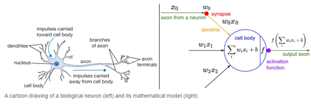
When comparing with a neuron-based model that is in our brains, the axon is at the end deciding what is to be transferred to the next neuron. That is exactly what an activation function does in an ANN as well. Hence it is also known as Transfer Function. It takes in the output signal from the previous cell and converts it into some form that can be taken as input to the next cell.

Why is there a need for it? Why use a non-linear activation function?

There are multiple reasons for having non-linear activation functions in a network.
Apart from the biological similarity that was discussed earlier, the most important feature in an activation function is its ability to add non-linearity into a neural network. To understand this, let’s consider multidimensional data. A linear classifier using three features can give us a line through the 3-D space but it will never be able to exactly learn the pattern because the pattern that defines this classification is not simply linear. If we use an ANN with a single cell but without an activation function. So our output is basically W*x + b. But this is no good because W*x also has a degree of 1, hence linear and this is basically identical to a linear classifier.

What if we stack multiple layers ?
No matter how many layers our neural network has, it will still behave just like a single layer network because summing these layers will give us another linear function which is not strong enough to model data.
```
  Let’s represent nᵗʰ layer as a linear function fₙ(x). So we have:
  o(x) = fₙ(fₙ₋₁(….f₁(x))
  If we take a 3 layer neural network with a linear function we get:
  o(x) = W3*(W2*(W1*x + b1) + b2) + b3
  This is equivalent to some W’*x + b’
  
```
“ A neural network without an activation function is just like a linear regression model.”

To give the model the power to learn the non-linear patterns and increase the degree of complexity, specific nonlinear layers called activation functions are added in between.
Back-propagation is not possible with linear functions as their derivative is constant, and has no relation to the input, X. So it’s not possible to go back and understand which weights in the input neurons can provide a better prediction. On the other hand nonlinear activation functions allow back-propagation because they have a derivative function which is related to the inputs.

Various Non-linear activation functions:-

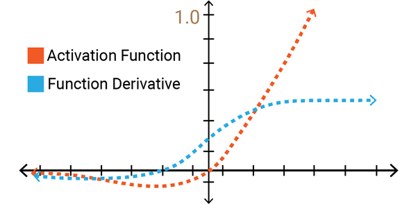
Sigmoid / Logistic Activation Function
The sigmoid function is well-known among the data science community because of its use in logistic regression, one of the core machine learning techniques used to solve classification problems.
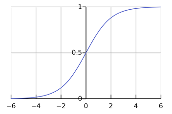
```
      Equation: s = 1/(1 + e-x)
      Derivative: f’(x) = s*(1-s)
      Value Range : 0 to 1
    
```
The Sigmoid Function curve looks like a S-shape.

The main reason why we use sigmoid function is because it exists between (0 to 1). Therefore, it is can be used for models where we have to predict the probability as an output. Since probability of anything exists only between the range of 0 and 1, sigmoid is the right choice.

Advantages
- The function is differentiable. That means, we can find the slope of the sigmoid curve at any two points.
- The function is monotonic but function’s derivative is not.
- Smooth gradient, preventing “jumps” in output values.
- Output values bound between 0 and 1, normalizing the output of each neuron.
Disadvantages
- Vanishing gradient—Sigmoids saturate for very high or very low values of X, there is almost no change to the prediction, causing a vanishing gradient problem. This can result in the network refusing to learn further, or being too slow to reach an accurate prediction.
- Outputs not zero centred makes the gradient updates go too far in different directions. 0 < output < 1, and it makes optimization harder.
- Computationally expensive as Sigmoid has slow convergence.
Uses:
Usually only used in the output layer of a binary classification, where result is either 0 or 1. The result can be predicted easily to be 1 if value is greater than threshold value and 0 otherwise.

SoftMax function is often described as a combination of multiple sigmoid. The SoftMax is a more generalised form of the sigmoid. It is used in multi-class classification problems.
Tanh / Hyperbolic Tangent Activation Function
The activation that almost always works better than sigmoid function is Tanh function also known as Tangent Hyperbolic function. It’s actually a mathematically shifted version of the sigmoid function. Both are similar and can be derived from each other.
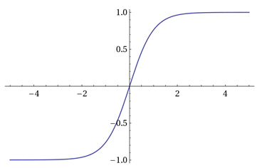
```
      Equation: f(x)= a = tanh(x) = 2/(1 + e-2x) - 1 = 2 * sigmoid(2x) - 1
      Derivative: (1- a²)
      Value Range: -1 to +1
    
```
Advantages:
- If you compare it to sigmoid, it solves just one problem of being Zero centred — making it easier to model inputs that have strongly negative, neutral, and strongly positive values.
- Works better than sigmoid function
Disadvantage:
- It also suffers from the vanishing gradient problem and hence slow convergence.
Uses:
Can be used in hidden layers of a neural network as it’s values lie between -1 to 1 hence the mean for the hidden layer is centred and comes out be 0 or very close to it. This makes learning for the next layer much easier.
ReLU
The Rectified Linear Unit is the most commonly used activation function in deep learning models. This simple function can allow the model to account for non-linearities and interactions well. Despite its name and appearance, it’s not linear and provides the same benefits as Sigmoid but with better performance. It can be written as f(x)=max(0,x). Graphically it looks like this.
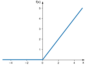
```
      Equation: f(x) = max(0,x)
      Derivative: f′(x)={ 1;x>0,
                          0;x<0 }
      Range: [ 0 to infinity)
    
```
The function and its derivative both are monotonic.

Advantages:
- It rectifies and avoids vanishing gradient problem.
- It is more computationally efficient to compute than Sigmoid like functions since Relu just needs to pick max(0, x) and not perform expensive exponential operations as in Sigmoids
- In practice, networks with Relu tend to show better convergence performance than sigmoid.
Disadvantages:
- Tend to blow up activation (there is no mechanism to constrain the output of the neuron, as "a" itself is the output)
- Dying Relu problem - if too many activations get below zero then most of the units(neurons) in network with Relu will simply output zero, in other words, die and thereby prohibiting learning.(This can be handled, to some extent, by using Leaky-Relu instead.)
- Non-differentiable at zero; however, it is differentiable anywhere else, and the value of the derivative at zero can be arbitrarily chosen to be 0 or 1.
- Bias Shift : From ReLU, there is a positive bias in the network for subsequent layers, as the mean activation is larger than zero. The positive mean shift in the next layers slows down learning.
- It can only be used within Hidden layers of a Neural Network Model.
Uses:
The rectified linear activation function overcomes the vanishing gradient problem, allowing models to learn faster and perform better. It is the default activation when developing multilayer Perceptron and convolutional neural networks.
Leaky ReLU
The Leaky ReLU (LReLU or LReL) modifies the function to allow small negative values when the input is less than zero. The leaky rectifier allows for a small, non-zero gradient when the unit is saturated and not active.
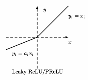
```
      Equation: R(z)={z;z>0,
                     αz;z<=0}
      Derivative: R′(z)={1;z>0,
                         α;z<0}
      Range: (-infinity to infinity)
    
```
Advantage:
- Leaky ReLUs are one attempt to fix the “dying ReLU” problem by having a small negative slope (of 0.01, or so).
Disadvantage:
- As it possess linearity, it can’t be used for the complex Classification. It lags behind the Sigmoid and Tanh for some of the use cases.
Uses:
Leaky ReLU has a small slope for negative values, instead of altogether zero. Leaky ReLU has two benefits: It fixes the “dying ReLU” problem, as it doesn't have zero-slope parts. It speeds up training.
Swish
Swish is a new, self-gated activation function discovered by researchers at Google. According to their paper, it performs better than ReLU with a similar level of computational efficiency. In experiments on ImageNet with identical models running ReLU and Swish, the new function achieved top -1 classification accuracy 0.6-0.9% higher.
```
      Equation: Y = X * sigmoid(X)
      Derivative: Y’ = Y + sigmoid(X) * (1-Y)
    
```
It is a non-monotonic function.

Advantages:
- No dying ReLU.
- Increase in accuracy over ReLU.
- Outperforms ReLU in every batch size.
Disadvantages:
- Slightly more computationally expensive
- More problems with the algorithm will probably arise given time

Activation Function In Neural Networks

What is an activation function ?

Why is there a need for it? Why use a non-linear activation function?

What if we stack multiple layers ?

Various Non-linear activation functions:-

Sigmoid / Logistic Activation Function

Advantages

Disadvantages

Uses:

Tanh / Hyperbolic Tangent Activation Function

Advantages:

Disadvantage:

Uses:

ReLU

Advantages:

Disadvantages:

Uses:

Leaky ReLU

Advantage:

Disadvantage:

Uses:

Swish

Advantages:

Disadvantages: